Multiple Stock Trading
Deep Reinforcement Learning for Stock Trading from Scratch: Multiple Stock Trading
Tip
Run the code step by step at Google Colab.
Step 1: Preparation
Step 1.1: Overview
To begin with, I would like explain the logic of multiple stock trading using Deep Reinforcement Learning.
We use Dow 30 constituents as an example throughout this article, because those are the most popular stocks.
A lot of people are terrified by the word “Deep Reinforcement Learning”, actually, you can just treat it as a “Smart AI” or “Smart Stock Trader” or “R2-D2 Trader” if you want, and just use it.
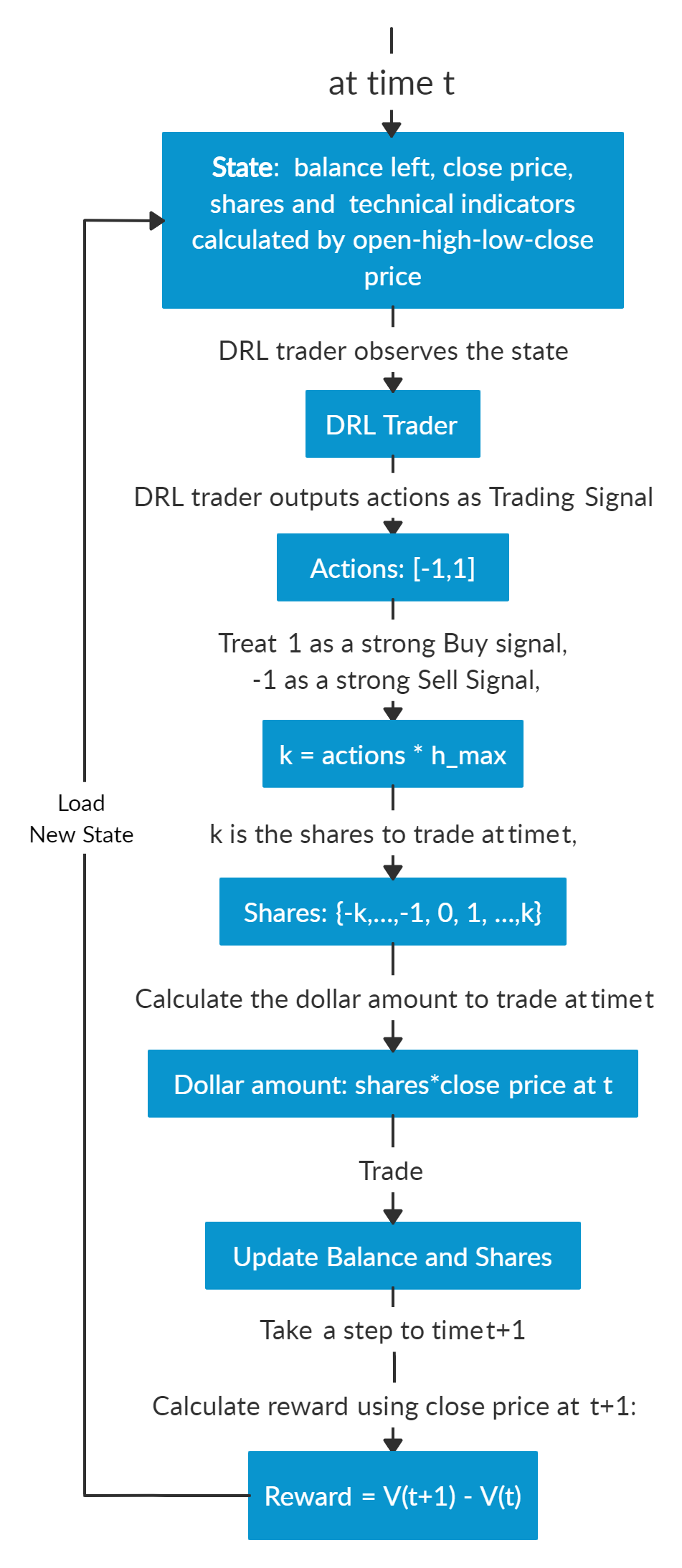
Suppose that we have a well trained DRL agent “DRL Trader”, we want to use it to trade multiple stocks in our portfolio.
Assume we are at time t, at the end of day at time t, we will know the open-high-low-close price of the Dow 30 constituents stocks. We can use these information to calculate technical indicators such as MACD, RSI, CCI, ADX. In Reinforcement Learning we call these data or features as “states”.
We know that our portfolio value V(t) = balance (t) + dollar amount of the stocks (t).
We feed the states into our well trained DRL Trader, the trader will output a list of actions, the action for each stock is a value within [-1, 1], we can treat this value as the trading signal, 1 means a strong buy signal, -1 means a strong sell signal.
We calculate k = actions *h_max, h_max is a predefined parameter that sets as the maximum amount of shares to trade. So we will have a list of shares to trade.
The dollar amount of shares = shares to trade* close price (t).
Update balance and shares. These dollar amount of shares are the money we need to trade at time t. The updated balance = balance (t) −amount of money we pay to buy shares +amount of money we receive to sell shares. The updated shares = shares held (t) −shares to sell +shares to buy.
So we take actions to trade based on the advice of our DRL Trader at the end of day at time t (time t’s close price equals time t+1’s open price). We hope that we will benefit from these actions by the end of day at time t+1.
Take a step to time t+1, at the end of day, we will know the close price at t+1, the dollar amount of the stocks (t+1)= sum(updated shares * close price (t+1)). The portfolio value V(t+1)=balance (t+1) + dollar amount of the stocks (t+1).
So the step reward by taking the actions from DRL Trader at time t to t+1 is r = v(t+1) − v(t). The reward can be positive or negative in the training stage. But of course, we need a positive reward in trading to say that our DRL Trader is effective.
Repeat this process until termination.
Below are the logic chart of multiple stock trading and a made-up example for demonstration purpose:

Multiple stock trading is different from single stock trading because as the number of stocks increase, the dimension of the data will increase, the state and action space in reinforcement learning will grow exponentially. So stability and reproducibility are very essential here.
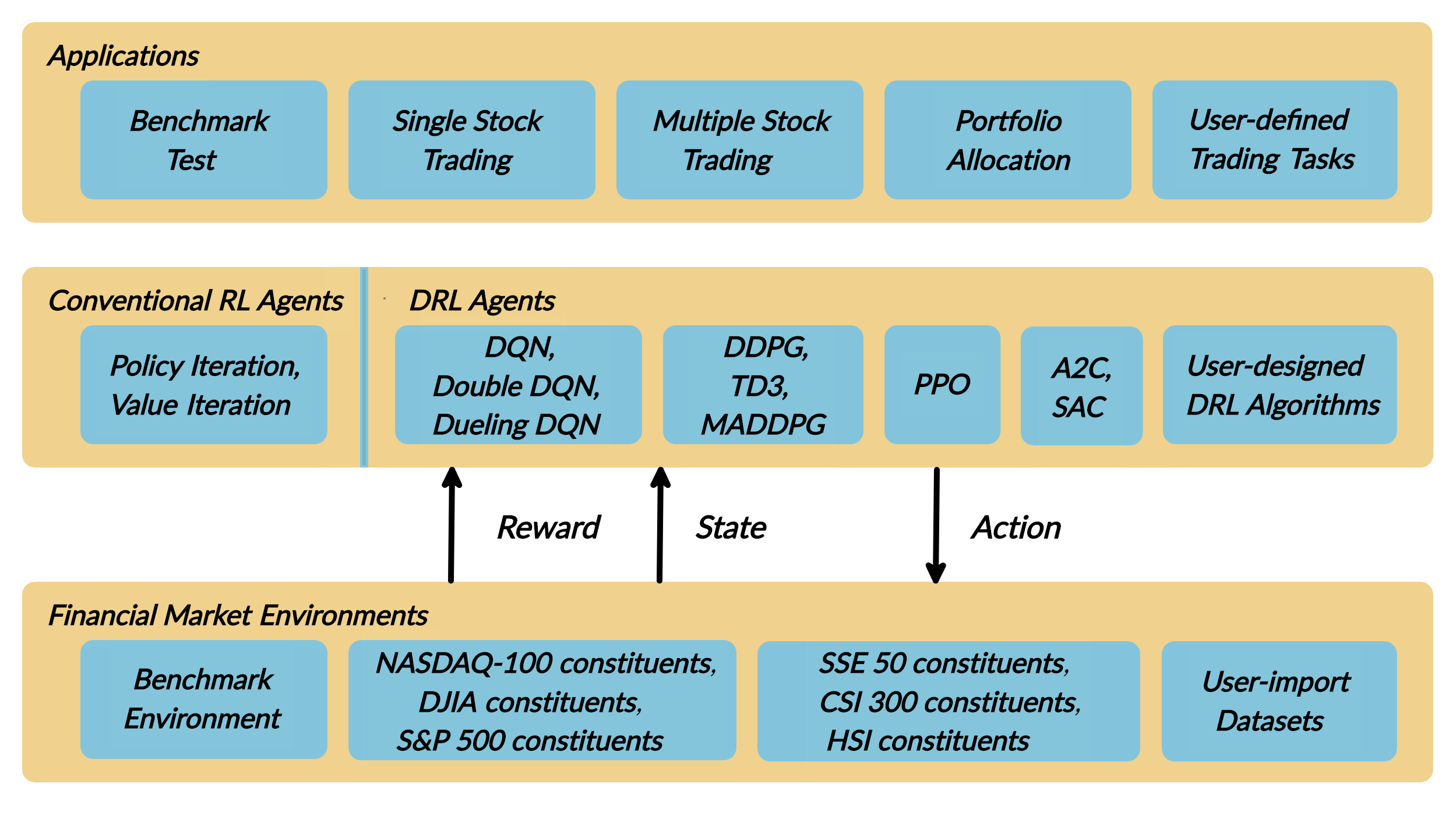
We introduce a DRL library FinRL that facilitates beginners to expose themselves to quantitative finance and to develop their own stock trading strategies.
FinRL is characterized by its reproducibility, scalability, simplicity, applicability and extendibility.
This article is focusing on one of the use cases in our paper: Mutiple Stock Trading. We use one Jupyter notebook to include all the necessary steps.
Step 1.2: Problem Definition:
This problem is to design an automated solution for stock trading. We model the stock trading process as a Markov Decision Process (MDP). We then formulate our trading goal as a maximization problem. The algorithm is trained using Deep Reinforcement Learning (DRL) algorithms and the components of the reinforcement learning environment are:
Action: The action space describes the allowed actions that the agent interacts with the environment. Normally, a ∈ A includes three actions: a ∈ {−1, 0, 1}, where −1, 0, 1 represent selling, holding, and buying one stock. Also, an action can be carried upon multiple shares. We use an action space {−k, …, −1, 0, 1, …, k}, where k denotes the number of shares. For example, “Buy 10 shares of AAPL” or “Sell 10 shares of AAPL” are 10 or −10, respectively
Reward function: r(s, a, s′) is the incentive mechanism for an agent to learn a better action. The change of the portfolio value when action a is taken at state s and arriving at new state s’, i.e., r(s, a, s′) = v′ − v, where v′ and v represent the portfolio values at state s′ and s, respectively
State: The state space describes the observations that the agent receives from the environment. Just as a human trader needs to analyze various information before executing a trade, so our trading agent observes many different features to better learn in an interactive environment.
Environment: Dow 30 constituents
The data of the stocks for this case study is obtained from Yahoo Finance API. The data contains Open-High-Low-Close price and volume.
Step 1.3: FinRL installation:
1## install finrl library
2!pip install git+https://github.com/AI4Finance-LLC/FinRL-Library.git
Then we import the packages needed for this demonstration.
Step 1.4: Import packages:
 1import pandas as pd
 2import numpy as np
 3import matplotlib
 4import matplotlib.pyplot as plt
 5# matplotlib.use('Agg')
 6import datetime
 7
 8%matplotlib inline
 9from finrl import config
10from finrl import config_tickers
11from finrl.finrl_meta.preprocessor.yahoodownloader import YahooDownloader
12from finrl.finrl_meta.preprocessor.preprocessors import FeatureEngineer, data_split
13from finrl.finrl_meta.env_stock_trading.env_stocktrading import StockTradingEnv
14from finrl.agents.stablebaselines3.models import DRLAgent
15
16from finrl.plot import backtest_stats, backtest_plot, get_daily_return, get_baseline
17from pprint import pprint
18
19import sys
20sys.path.append("../FinRL-Library")
21
22import itertools
Finally, create folders for storage.
Step 1.5: Create folders:
1import os
2if not os.path.exists("./" + config.DATA_SAVE_DIR):
3    os.makedirs("./" + config.DATA_SAVE_DIR)
4if not os.path.exists("./" + config.TRAINED_MODEL_DIR):
5    os.makedirs("./" + config.TRAINED_MODEL_DIR)
6if not os.path.exists("./" + config.TENSORBOARD_LOG_DIR):
7    os.makedirs("./" + config.TENSORBOARD_LOG_DIR)
8if not os.path.exists("./" + config.RESULTS_DIR):
9    os.makedirs("./" + config.RESULTS_DIR)
Then all the preparation work are done. We can start now!
Step 2: Download Data
Before training our DRL agent, we need to get the historical data of DOW30 stocks first. Here we use the data from Yahoo! Finance. Yahoo! Finance is a website that provides stock data, financial news, financial reports, etc. All the data provided by Yahoo Finance is free. yfinance is an open-source library that provides APIs to download data from Yahoo! Finance. We will use this package to download data here.
FinRL uses a YahooDownloader class to extract data.
class YahooDownloader:
    """
    Provides methods for retrieving daily stock data from Yahoo Finance API

    Attributes
    ----------
        start_date : str
            start date of the data (modified from config.py)
        end_date : str
            end date of the data (modified from config.py)
        ticker_list : list
            a list of stock tickers (modified from config.py)

    Methods
    -------
        fetch_data()
            Fetches data from yahoo API
    """
Download and save the data in a pandas DataFrame:
1 # Download and save the data in a pandas DataFrame:
2 df = YahooDownloader(start_date = '2009-01-01',
3                           end_date = '2020-09-30',
4                           ticker_list = config_tickers.DOW_30_TICKER).fetch_data()
5
6 print(df.sort_values(['date','tic'],ignore_index=True).head(30))

Step 3: Preprocess Data
Data preprocessing is a crucial step for training a high quality machine learning model. We need to check for missing data and do feature engineering in order to convert the data into a model-ready state.
Step 3.1: Check missing data
1# check missing data
2dow_30.isnull().values.any()
Step 3.2: Add technical indicators
In practical trading, various information needs to be taken into account, for example the historical stock prices, current holding shares, technical indicators, etc. In this article, we demonstrate two trend-following technical indicators: MACD and RSI.
 1def add_technical_indicator(df):
 2        """
 3        calcualte technical indicators
 4        use stockstats package to add technical inidactors
 5        :param data: (df) pandas dataframe
 6        :return: (df) pandas dataframe
 7        """
 8        stock = Sdf.retype(df.copy())
 9        stock['close'] = stock['adjcp']
10        unique_ticker = stock.tic.unique()
11
12        macd = pd.DataFrame()
13        rsi = pd.DataFrame()
14
15        #temp = stock[stock.tic == unique_ticker[0]]['macd']
16        for i in range(len(unique_ticker)):
17            ## macd
18            temp_macd = stock[stock.tic == unique_ticker[i]]['macd']
19            temp_macd = pd.DataFrame(temp_macd)
20            macd = macd.append(temp_macd, ignore_index=True)
21            ## rsi
22            temp_rsi = stock[stock.tic == unique_ticker[i]]['rsi_30']
23            temp_rsi = pd.DataFrame(temp_rsi)
24            rsi = rsi.append(temp_rsi, ignore_index=True)
25
26        df['macd'] = macd
27        df['rsi'] = rsi
28        return df
Step 3.3: Add turbulence index
Risk-aversion reflects whether an investor will choose to preserve the capital. It also influences one’s trading strategy when facing different market volatility level.
To control the risk in a worst-case scenario, such as financial crisis of 2007–2008, FinRL employs the financial turbulence index that measures extreme asset price fluctuation.
 1def add_turbulence(df):
 2    """
 3    add turbulence index from a precalcualted dataframe
 4    :param data: (df) pandas dataframe
 5    :return: (df) pandas dataframe
 6    """
 7    turbulence_index = calcualte_turbulence(df)
 8    df = df.merge(turbulence_index, on='datadate')
 9    df = df.sort_values(['datadate','tic']).reset_index(drop=True)
10    return df
11
12
13
14def calcualte_turbulence(df):
15    """calculate turbulence index based on dow 30"""
16    # can add other market assets
17
18    df_price_pivot=df.pivot(index='datadate', columns='tic', values='adjcp')
19    unique_date = df.datadate.unique()
20    # start after a year
21    start = 252
22    turbulence_index = [0]*start
23    #turbulence_index = [0]
24    count=0
25    for i in range(start,len(unique_date)):
26        current_price = df_price_pivot[df_price_pivot.index == unique_date[i]]
27        hist_price = df_price_pivot[[n in unique_date[0:i] for n in df_price_pivot.index ]]
28        cov_temp = hist_price.cov()
29        current_temp=(current_price - np.mean(hist_price,axis=0))
30        temp = current_temp.values.dot(np.linalg.inv(cov_temp)).dot(current_temp.values.T)
31        if temp>0:
32            count+=1
33            if count>2:
34                turbulence_temp = temp[0][0]
35            else:
36                #avoid large outlier because of the calculation just begins
37                turbulence_temp=0
38        else:
39            turbulence_temp=0
40        turbulence_index.append(turbulence_temp)
41
42
43    turbulence_index = pd.DataFrame({'datadate':df_price_pivot.index,
44                                     'turbulence':turbulence_index})
45    return turbulence_index
Step 3.4 Feature Engineering
FinRL uses a FeatureEngineer class to preprocess data.
Perform Feature Engineering:
1 # Perform Feature Engineering:
2 df = FeatureEngineer(df.copy(),
3                      use_technical_indicator=True,
4                      tech_indicator_list = config.INDICATORS,
5                      use_turbulence=True,
6                      user_defined_feature = False).preprocess_data()

Step 4: Design Environment
Considering the stochastic and interactive nature of the automated stock trading tasks, a financial task is modeled as a Markov Decision Process (MDP) problem. The training process involves observing stock price change, taking an action and reward’s calculation to have the agent adjusting its strategy accordingly. By interacting with the environment, the trading agent will derive a trading strategy with the maximized rewards as time proceeds.
Our trading environments, based on OpenAI Gym framework, simulate live stock markets with real market data according to the principle of time-driven simulation.
The action space describes the allowed actions that the agent interacts with the environment. Normally, action a includes three actions: {-1, 0, 1}, where -1, 0, 1 represent selling, holding, and buying one share. Also, an action can be carried upon multiple shares. We use an action space {-k,…,-1, 0, 1, …, k}, where k denotes the number of shares to buy and -k denotes the number of shares to sell. For example, “Buy 10 shares of AAPL” or “Sell 10 shares of AAPL” are 10 or -10, respectively. The continuous action space needs to be normalized to [-1, 1], since the policy is defined on a Gaussian distribution, which needs to be normalized and symmetric.
Step 4.1: Environment for Training
  1## Environment for Training
  2import numpy as np
  3import pandas as pd
  4from gym.utils import seeding
  5import gym
  6from gym import spaces
  7import matplotlib
  8matplotlib.use('Agg')
  9import matplotlib.pyplot as plt
 10
 11# shares normalization factor
 12# 100 shares per trade
 13HMAX_NORMALIZE = 100
 14# initial amount of money we have in our account
 15INITIAL_ACCOUNT_BALANCE=1000000
 16# total number of stocks in our portfolio
 17STOCK_DIM = 30
 18# transaction fee: 1/1000 reasonable percentage
 19TRANSACTION_FEE_PERCENT = 0.001
 20
 21REWARD_SCALING = 1e-4
 22
 23
 24class StockEnvTrain(gym.Env):
 25    """A stock trading environment for OpenAI gym"""
 26    metadata = {'render.modes': ['human']}
 27
 28    def __init__(self, df,day = 0):
 29        #super(StockEnv, self).__init__()
 30        self.day = day
 31        self.df = df
 32
 33        # action_space normalization and shape is STOCK_DIM
 34        self.action_space = spaces.Box(low = -1, high = 1,shape = (STOCK_DIM,))
 35        # Shape = 181: [Current Balance]+[prices 1-30]+[owned shares 1-30]
 36        # +[macd 1-30]+ [rsi 1-30] + [cci 1-30] + [adx 1-30]
 37        self.observation_space = spaces.Box(low=0, high=np.inf, shape = (121,))
 38        # load data from a pandas dataframe
 39        self.data = self.df.loc[self.day,:]
 40        self.terminal = False
 41        # initalize state
 42        self.state = [INITIAL_ACCOUNT_BALANCE] + \
 43                      self.data.adjcp.values.tolist() + \
 44                      [0]*STOCK_DIM + \
 45                      self.data.macd.values.tolist() + \
 46                      self.data.rsi.values.tolist()
 47                      #self.data.cci.values.tolist() + \
 48                      #self.data.adx.values.tolist()
 49        # initialize reward
 50        self.reward = 0
 51        self.cost = 0
 52        # memorize all the total balance change
 53        self.asset_memory = [INITIAL_ACCOUNT_BALANCE]
 54        self.rewards_memory = []
 55        self.trades = 0
 56        self._seed()
 57
 58    def _sell_stock(self, index, action):
 59        # perform sell action based on the sign of the action
 60        if self.state[index+STOCK_DIM+1] > 0:
 61            #update balance
 62            self.state[0] += \
 63            self.state[index+1]*min(abs(action),self.state[index+STOCK_DIM+1]) * \
 64             (1- TRANSACTION_FEE_PERCENT)
 65
 66            self.state[index+STOCK_DIM+1] -= min(abs(action), self.state[index+STOCK_DIM+1])
 67            self.cost +=self.state[index+1]*min(abs(action),self.state[index+STOCK_DIM+1]) * \
 68             TRANSACTION_FEE_PERCENT
 69            self.trades+=1
 70        else:
 71            pass
 72
 73    def _buy_stock(self, index, action):
 74        # perform buy action based on the sign of the action
 75        available_amount = self.state[0] // self.state[index+1]
 76        # print('available_amount:{}'.format(available_amount))
 77
 78        #update balance
 79        self.state[0] -= self.state[index+1]*min(available_amount, action)* \
 80                          (1+ TRANSACTION_FEE_PERCENT)
 81
 82        self.state[index+STOCK_DIM+1] += min(available_amount, action)
 83
 84        self.cost+=self.state[index+1]*min(available_amount, action)* \
 85                          TRANSACTION_FEE_PERCENT
 86        self.trades+=1
 87
 88    def step(self, actions):
 89        # print(self.day)
 90        self.terminal = self.day >= len(self.df.index.unique())-1
 91        # print(actions)
 92
 93        if self.terminal:
 94            plt.plot(self.asset_memory,'r')
 95            plt.savefig('account_value_train.png')
 96            plt.close()
 97            end_total_asset = self.state[0]+ \
 98            sum(np.array(self.state[1:(STOCK_DIM+1)])*np.array(self.state[(STOCK_DIM+1):(STOCK_DIM*2+1)]))
 99            print("previous_total_asset:{}".format(self.asset_memory[0]))
100
101            print("end_total_asset:{}".format(end_total_asset))
102            df_total_value = pd.DataFrame(self.asset_memory)
103            df_total_value.to_csv('account_value_train.csv')
104            print("total_reward:{}".format(self.state[0]+sum(np.array(self.state[1:(STOCK_DIM+1)])*np.array(self.state[(STOCK_DIM+1):61]))- INITIAL_ACCOUNT_BALANCE ))
105            print("total_cost: ", self.cost)
106            print("total_trades: ", self.trades)
107            df_total_value.columns = ['account_value']
108            df_total_value['daily_return']=df_total_value.pct_change(1)
109            sharpe = (252**0.5)*df_total_value['daily_return'].mean()/ \
110                  df_total_value['daily_return'].std()
111            print("Sharpe: ",sharpe)
112            print("=================================")
113            df_rewards = pd.DataFrame(self.rewards_memory)
114            df_rewards.to_csv('account_rewards_train.csv')
115
116            return self.state, self.reward, self.terminal,{}
117
118        else:
119            actions = actions * HMAX_NORMALIZE
120
121            begin_total_asset = self.state[0]+ \
122            sum(np.array(self.state[1:(STOCK_DIM+1)])*np.array(self.state[(STOCK_DIM+1):61]))
123            #print("begin_total_asset:{}".format(begin_total_asset))
124
125            argsort_actions = np.argsort(actions)
126
127            sell_index = argsort_actions[:np.where(actions < 0)[0].shape[0]]
128            buy_index = argsort_actions[::-1][:np.where(actions > 0)[0].shape[0]]
129
130            for index in sell_index:
131                # print('take sell action'.format(actions[index]))
132                self._sell_stock(index, actions[index])
133
134            for index in buy_index:
135                # print('take buy action: {}'.format(actions[index]))
136                self._buy_stock(index, actions[index])
137
138            self.day += 1
139            self.data = self.df.loc[self.day,:]
140            #load next state
141            # print("stock_shares:{}".format(self.state[29:]))
142            self.state =  [self.state[0]] + \
143                    self.data.adjcp.values.tolist() + \
144                    list(self.state[(STOCK_DIM+1):61]) + \
145                    self.data.macd.values.tolist() + \
146                    self.data.rsi.values.tolist()
147
148            end_total_asset = self.state[0]+ \
149            sum(np.array(self.state[1:(STOCK_DIM+1)])*np.array(self.state[(STOCK_DIM+1):61]))
150
151            #print("end_total_asset:{}".format(end_total_asset))
152
153            self.reward = end_total_asset - begin_total_asset
154            self.rewards_memory.append(self.reward)
155
156            self.reward = self.reward * REWARD_SCALING
157            # print("step_reward:{}".format(self.reward))
158
159            self.asset_memory.append(end_total_asset)
160
161
162        return self.state, self.reward, self.terminal, {}
163
164    def reset(self):
165        self.asset_memory = [INITIAL_ACCOUNT_BALANCE]
166        self.day = 0
167        self.data = self.df.loc[self.day,:]
168        self.cost = 0
169        self.trades = 0
170        self.terminal = False
171        self.rewards_memory = []
172        #initiate state
173        self.state = [INITIAL_ACCOUNT_BALANCE] + \
174                      self.data.adjcp.values.tolist() + \
175                      [0]*STOCK_DIM + \
176                      self.data.macd.values.tolist() + \
177                      self.data.rsi.values.tolist()
178        return self.state
179
180    def render(self, mode='human'):
181        return self.state
182
183    def _seed(self, seed=None):
184        self.np_random, seed = seeding.np_random(seed)
185        return [seed]
Step 4.2: Environment for Trading
  1## Environment for Trading
  2import numpy as np
  3import pandas as pd
  4from gym.utils import seeding
  5import gym
  6from gym import spaces
  7import matplotlib
  8matplotlib.use('Agg')
  9import matplotlib.pyplot as plt
 10
 11# shares normalization factor
 12# 100 shares per trade
 13HMAX_NORMALIZE = 100
 14# initial amount of money we have in our account
 15INITIAL_ACCOUNT_BALANCE=1000000
 16# total number of stocks in our portfolio
 17STOCK_DIM = 30
 18# transaction fee: 1/1000 reasonable percentage
 19TRANSACTION_FEE_PERCENT = 0.001
 20
 21# turbulence index: 90-150 reasonable threshold
 22#TURBULENCE_THRESHOLD = 140
 23REWARD_SCALING = 1e-4
 24
 25class StockEnvTrade(gym.Env):
 26    """A stock trading environment for OpenAI gym"""
 27    metadata = {'render.modes': ['human']}
 28
 29    def __init__(self, df,day = 0,turbulence_threshold=140):
 30        #super(StockEnv, self).__init__()
 31        #money = 10 , scope = 1
 32        self.day = day
 33        self.df = df
 34        # action_space normalization and shape is STOCK_DIM
 35        self.action_space = spaces.Box(low = -1, high = 1,shape = (STOCK_DIM,))
 36        # Shape = 181: [Current Balance]+[prices 1-30]+[owned shares 1-30]
 37        # +[macd 1-30]+ [rsi 1-30] + [cci 1-30] + [adx 1-30]
 38        self.observation_space = spaces.Box(low=0, high=np.inf, shape = (121,))
 39        # load data from a pandas dataframe
 40        self.data = self.df.loc[self.day,:]
 41        self.terminal = False
 42        self.turbulence_threshold = turbulence_threshold
 43        # initalize state
 44        self.state = [INITIAL_ACCOUNT_BALANCE] + \
 45                      self.data.adjcp.values.tolist() + \
 46                      [0]*STOCK_DIM + \
 47                      self.data.macd.values.tolist() + \
 48                      self.data.rsi.values.tolist()
 49
 50        # initialize reward
 51        self.reward = 0
 52        self.turbulence = 0
 53        self.cost = 0
 54        self.trades = 0
 55        # memorize all the total balance change
 56        self.asset_memory = [INITIAL_ACCOUNT_BALANCE]
 57        self.rewards_memory = []
 58        self.actions_memory=[]
 59        self.date_memory=[]
 60        self._seed()
 61
 62
 63    def _sell_stock(self, index, action):
 64        # perform sell action based on the sign of the action
 65        if self.turbulence<self.turbulence_threshold:
 66            if self.state[index+STOCK_DIM+1] > 0:
 67                #update balance
 68                self.state[0] += \
 69                self.state[index+1]*min(abs(action),self.state[index+STOCK_DIM+1]) * \
 70                 (1- TRANSACTION_FEE_PERCENT)
 71
 72                self.state[index+STOCK_DIM+1] -= min(abs(action), self.state[index+STOCK_DIM+1])
 73                self.cost +=self.state[index+1]*min(abs(action),self.state[index+STOCK_DIM+1]) * \
 74                 TRANSACTION_FEE_PERCENT
 75                self.trades+=1
 76            else:
 77                pass
 78        else:
 79            # if turbulence goes over threshold, just clear out all positions
 80            if self.state[index+STOCK_DIM+1] > 0:
 81                #update balance
 82                self.state[0] += self.state[index+1]*self.state[index+STOCK_DIM+1]* \
 83                              (1- TRANSACTION_FEE_PERCENT)
 84                self.state[index+STOCK_DIM+1] =0
 85                self.cost += self.state[index+1]*self.state[index+STOCK_DIM+1]* \
 86                              TRANSACTION_FEE_PERCENT
 87                self.trades+=1
 88            else:
 89                pass
 90
 91    def _buy_stock(self, index, action):
 92        # perform buy action based on the sign of the action
 93        if self.turbulence< self.turbulence_threshold:
 94            available_amount = self.state[0] // self.state[index+1]
 95            # print('available_amount:{}'.format(available_amount))
 96
 97            #update balance
 98            self.state[0] -= self.state[index+1]*min(available_amount, action)* \
 99                              (1+ TRANSACTION_FEE_PERCENT)
100
101            self.state[index+STOCK_DIM+1] += min(available_amount, action)
102
103            self.cost+=self.state[index+1]*min(available_amount, action)* \
104                              TRANSACTION_FEE_PERCENT
105            self.trades+=1
106        else:
107            # if turbulence goes over threshold, just stop buying
108            pass
109
110    def step(self, actions):
111        # print(self.day)
112        self.terminal = self.day >= len(self.df.index.unique())-1
113        # print(actions)
114
115        if self.terminal:
116            plt.plot(self.asset_memory,'r')
117            plt.savefig('account_value_trade.png')
118            plt.close()
119
120            df_date = pd.DataFrame(self.date_memory)
121            df_date.columns = ['datadate']
122            df_date.to_csv('df_date.csv')
123
124
125            df_actions = pd.DataFrame(self.actions_memory)
126            df_actions.columns = self.data.tic.values
127            df_actions.index = df_date.datadate
128            df_actions.to_csv('df_actions.csv')
129
130            df_total_value = pd.DataFrame(self.asset_memory)
131            df_total_value.to_csv('account_value_trade.csv')
132            end_total_asset = self.state[0]+ \
133            sum(np.array(self.state[1:(STOCK_DIM+1)])*np.array(self.state[(STOCK_DIM+1):(STOCK_DIM*2+1)]))
134            print("previous_total_asset:{}".format(self.asset_memory[0]))
135
136            print("end_total_asset:{}".format(end_total_asset))
137            print("total_reward:{}".format(self.state[0]+sum(np.array(self.state[1:(STOCK_DIM+1)])*np.array(self.state[(STOCK_DIM+1):61]))- self.asset_memory[0] ))
138            print("total_cost: ", self.cost)
139            print("total trades: ", self.trades)
140
141            df_total_value.columns = ['account_value']
142            df_total_value['daily_return']=df_total_value.pct_change(1)
143            sharpe = (252**0.5)*df_total_value['daily_return'].mean()/ \
144                  df_total_value['daily_return'].std()
145            print("Sharpe: ",sharpe)
146
147            df_rewards = pd.DataFrame(self.rewards_memory)
148            df_rewards.to_csv('account_rewards_trade.csv')
149
150            # print('total asset: {}'.format(self.state[0]+ sum(np.array(self.state[1:29])*np.array(self.state[29:]))))
151            #with open('obs.pkl', 'wb') as f:
152            #    pickle.dump(self.state, f)
153
154            return self.state, self.reward, self.terminal,{}
155
156        else:
157            # print(np.array(self.state[1:29]))
158            self.date_memory.append(self.data.datadate.unique())
159
160            #print(self.data)
161            actions = actions * HMAX_NORMALIZE
162            if self.turbulence>=self.turbulence_threshold:
163                actions=np.array([-HMAX_NORMALIZE]*STOCK_DIM)
164            self.actions_memory.append(actions)
165
166            #actions = (actions.astype(int))
167
168            begin_total_asset = self.state[0]+ \
169            sum(np.array(self.state[1:(STOCK_DIM+1)])*np.array(self.state[(STOCK_DIM+1):(STOCK_DIM*2+1)]))
170            #print("begin_total_asset:{}".format(begin_total_asset))
171
172            argsort_actions = np.argsort(actions)
173            #print(argsort_actions)
174
175            sell_index = argsort_actions[:np.where(actions < 0)[0].shape[0]]
176            buy_index = argsort_actions[::-1][:np.where(actions > 0)[0].shape[0]]
177
178            for index in sell_index:
179                # print('take sell action'.format(actions[index]))
180                self._sell_stock(index, actions[index])
181
182            for index in buy_index:
183                # print('take buy action: {}'.format(actions[index]))
184                self._buy_stock(index, actions[index])
185
186            self.day += 1
187            self.data = self.df.loc[self.day,:]
188            self.turbulence = self.data['turbulence'].values[0]
189            #print(self.turbulence)
190            #load next state
191            # print("stock_shares:{}".format(self.state[29:]))
192            self.state =  [self.state[0]] + \
193                    self.data.adjcp.values.tolist() + \
194                    list(self.state[(STOCK_DIM+1):(STOCK_DIM*2+1)]) + \
195                    self.data.macd.values.tolist() + \
196                    self.data.rsi.values.tolist()
197
198            end_total_asset = self.state[0]+ \
199            sum(np.array(self.state[1:(STOCK_DIM+1)])*np.array(self.state[(STOCK_DIM+1):(STOCK_DIM*2+1)]))
200
201            #print("end_total_asset:{}".format(end_total_asset))
202
203            self.reward = end_total_asset - begin_total_asset
204            self.rewards_memory.append(self.reward)
205
206            self.reward = self.reward * REWARD_SCALING
207
208            self.asset_memory.append(end_total_asset)
209
210        return self.state, self.reward, self.terminal, {}
211
212    def reset(self):
213        self.asset_memory = [INITIAL_ACCOUNT_BALANCE]
214        self.day = 0
215        self.data = self.df.loc[self.day,:]
216        self.turbulence = 0
217        self.cost = 0
218        self.trades = 0
219        self.terminal = False
220        #self.iteration=self.iteration
221        self.rewards_memory = []
222        self.actions_memory=[]
223        self.date_memory=[]
224        #initiate state
225        self.state = [INITIAL_ACCOUNT_BALANCE] + \
226                      self.data.adjcp.values.tolist() + \
227                      [0]*STOCK_DIM + \
228                      self.data.macd.values.tolist() + \
229                      self.data.rsi.values.tolist()
230
231        return self.state
232
233    def render(self, mode='human',close=False):
234        return self.state
235
236
237    def _seed(self, seed=None):
238        self.np_random, seed = seeding.np_random(seed)
239        return [seed]
Step 5: Implement DRL Algorithms
The implementation of the DRL algorithms are based on OpenAI Baselines and Stable Baselines. Stable Baselines is a fork of OpenAI Baselines, with a major structural refactoring, and code cleanups.
Step 5.1: Training data split: 2009-01-01 to 2018-12-31
 1def data_split(df,start,end):
 2    """
 3    split the dataset into training or testing using date
 4    :param data: (df) pandas dataframe, start, end
 5    :return: (df) pandas dataframe
 6    """
 7    data = df[(df.datadate >= start) & (df.datadate < end)]
 8    data=data.sort_values(['datadate','tic'],ignore_index=True)
 9    data.index = data.datadate.factorize()[0]
10    return data
Step 5.2: Model training: DDPG
 1## tensorboard --logdir ./multiple_stock_tensorboard/
 2# add noise to the action in DDPG helps in learning for better exploration
 3n_actions = env_train.action_space.shape[-1]
 4param_noise = None
 5action_noise = OrnsteinUhlenbeckActionNoise(mean=np.zeros(n_actions), sigma=float(0.5) * np.ones(n_actions))
 6
 7# model settings
 8model_ddpg = DDPG('MlpPolicy',
 9                   env_train,
10                   batch_size=64,
11                   buffer_size=100000,
12                   param_noise=param_noise,
13                   action_noise=action_noise,
14                   verbose=0,
15                   tensorboard_log="./multiple_stock_tensorboard/")
16
17## 250k timesteps: took about 20 mins to finish
18model_ddpg.learn(total_timesteps=250000, tb_log_name="DDPG_run_1")
Step 5.3: Trading
Assume that we have $1,000,000 initial capital at 2019-01-01. We use the DDPG model to trade Dow jones 30 stocks.
Step 5.4: Set turbulence threshold
Set the turbulence threshold to be the 99% quantile of insample turbulence data, if current turbulence index is greater than the threshold, then we assume that the current market is volatile
1insample_turbulence = dow_30[(dow_30.datadate<'2019-01-01') & (dow_30.datadate>='2009-01-01')]
2insample_turbulence = insample_turbulence.drop_duplicates(subset=['datadate'])
Step 5.5: Prepare test data and environment
1# test data
2test = data_split(dow_30, start='2019-01-01', end='2020-10-30')
3# testing env
4env_test = DummyVecEnv([lambda: StockEnvTrade(test, turbulence_threshold=insample_turbulence_threshold)])
5obs_test = env_test.reset()
Step 5.6: Prediction
1def DRL_prediction(model, data, env, obs):
2    print("==============Model Prediction===========")
3    for i in range(len(data.index.unique())):
4        action, _states = model.predict(obs)
5        obs, rewards, dones, info = env.step(action)
6        env.render()
Step 6: Backtest Our Strategy
For simplicity purposes, in the article, we just calculate the Sharpe ratio and the annual return manually.
1def backtest_strat(df):
2    strategy_ret= df.copy()
3    strategy_ret['Date'] = pd.to_datetime(strategy_ret['Date'])
4    strategy_ret.set_index('Date', drop = False, inplace = True)
5    strategy_ret.index = strategy_ret.index.tz_localize('UTC')
6    del strategy_ret['Date']
7    ts = pd.Series(strategy_ret['daily_return'].values, index=strategy_ret.index)
8    return ts
Step 6.1: Dow Jones Industrial Average
1def get_buy_and_hold_sharpe(test):
2    test['daily_return']=test['adjcp'].pct_change(1)
3    sharpe = (252**0.5)*test['daily_return'].mean()/ \
4    test['daily_return'].std()
5    annual_return = ((test['daily_return'].mean()+1)**252-1)*100
6    print("annual return: ", annual_return)
7
8    print("sharpe ratio: ", sharpe)
9    #return sharpe
Step 6.2: Our DRL trading strategy
 1def get_daily_return(df):
 2    df['daily_return']=df.account_value.pct_change(1)
 3    #df=df.dropna()
 4    sharpe = (252**0.5)*df['daily_return'].mean()/ \
 5    df['daily_return'].std()
 6
 7    annual_return = ((df['daily_return'].mean()+1)**252-1)*100
 8    print("annual return: ", annual_return)
 9    print("sharpe ratio: ", sharpe)
10    return df
Step 6.3: Plot the results using Quantopian pyfolio
Backtesting plays a key role in evaluating the performance of a trading strategy. Automated backtesting tool is preferred because it reduces the human error. We usually use the Quantopian pyfolio package to backtest our trading strategies. It is easy to use and consists of various individual plots that provide a comprehensive image of the performance of a trading strategy.
1%matplotlib inline
2with pyfolio.plotting.plotting_context(font_scale=1.1):
3    pyfolio.create_full_tear_sheet(returns = DRL_strat,
4                                   benchmark_rets=dow_strat, set_context=False)